Measuring Small-Beam MFD Overcoming the Challenges

Small beams are used in many critical applications yet often they are not directly profiled. While obtaining good beam profiling data on beams under 10 μm has its challenges, they can be overcome with proven techniques.

Author:

Derrick Peterman, PhD Ophir-Spiricon LLC

Profiling beams under 10 μm in size is one of the more challenging beam profiling applications. There are numerous reasons for this, including the very small size. Focal plane arrays commonly used in beam profiling have pixel dimensions of 3 to 10 μm, which are too large to reasonably profile these small beams without magnification. Further complicating these measurements are the high mechanical precision of the beam profiling apparatus, as well as the beams’ high divergences and rapid expansion.

These issues cause many organizations to “fly blind” on projects involving small beam sizes. Instead of using data from direct beam measurements, users typically rely on indirect methods and estimation, theoretical models, or the expectation that the vendor’s data actually reflects reality. Accurate beam size measurements at these sizes are critical in applications such as fiber optic coupling efficiency, defect scanning, optical design and optical fabrication process control.

While measuring a beam under 10 μm is more difficult than measuring a beam of 1 to 2 mm, reliable profiles of these small beams can be obtained in a straightforward manner. Two techniques commonly used are near-field profiling and far-field profiling. Near-field profiling seems obvious, as it involves imaging the light at its smallest point at the “near-field” of the beam waist. Far-field profiling is counterintuitive, in that the beam is analyzed at a great distance from the beam waist to determine its size; this type of profiling can be more advantageous than direct nearfield methods.

Where is the near-field and how is it profiled?

The near-field of a laser beam is the region around its beam waist, or focus. For small beams, a near-field profiler consists of a microscope objective lens to image and magnify the beam at its focus; the resulting image is captured with a beam profiler. In most cases, a CCD beam profiler is used, but it is also possible to use scanning aperture profilers. An important consideration in near-field profiling is the mechanical precision of positioning the apparatus, as the beam size measurements are sensitive to small imprecision in the image plane. We can understand the mechanical positioning constraints from the following beam propagation equation:

where Dz is the beam size at location z along the optical path, D0 is the beam waist (what is to be measured), and θ is the far-field beam divergence in radians. For a diffraction-limited beam, this becomes:

To determine precisely how the measurement plane needs to be established to measure a 5-μm beam within 2 percent accuracy for a beam at visible wavelengths, we use this equation to calculate it in the range of 5 to 7 μm. That means the entire apparatus must be positioned to this accuracy, relative to the focal point, to achieve a reasonably accurate beam size, and the depth of focus of the microscope objective lens must also be equally narrow (Figure 1). Mechanical positioning equipment and microscope objectives that meet the required precision are readily available.

Figure 1. A C-mount near-field profiler adapter assembly is commonly used in beam measurement.

Another important consideration is to ensure the beam attenuation is inserted where the beam is collimated – between the microscope objective lens and the beam profiler. Filters and beam attenuators near the beam focus create problems due to the large power and energy densities near the focus, which result in thermal lensing. Also, large divergence angles of the beam near the focus create distortions as the beam passes through the filter.

Another important consideration is to ensure the beam attenuation is inserted where the beam is collimated – between the microscope objective lens and the beam profiler. Filters and beam attenuators near the beam focus create problems due to the large power and energy densities near the focus, which result in thermal lensing. Also, large divergence angles of the beam near the focus create distortions as the beam passes through the filter.

Film Defect Inspection

Near-field profiling has been used to analyze optics in a film defect inspection system. The lenses were designed to produce 1- to 4-μm spot sizes on the test surface, coupled with adaptive optics to minimize distortions. In one lens, a beam spot size of about 2 μm was measured; a “halo” was observed around the beam in the profile (Figure 2), which degrades the resolution of the defect inspection system.

Figure 2. A 2-μm beam with little adaptive optic correction.

of the defect inspection system. However, using an adaptive optics routine, the halo was observed to be reduced (Figure 3).

Figure 3. A 2-μm beam with greater optic correction.

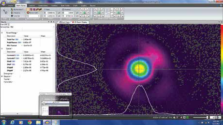
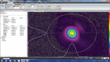
This comparison shows one of the strengths of using a focal plane array profiler with this technique. Since a focal plane array generates a 2D image of the profile, spatial features are easily observed. This often indicates the overall performance of the optics and also reveals optical defects that can degrade the performance of the optical system.

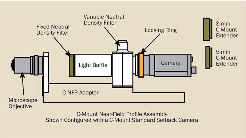
Scanning aperture profilers can measure beams under 10 μm, depending on their design, without the need for a microscope objective. This can make scanning aperture profiles seem attractive for measuring small beams, since the measurements are simplified; scanning aperture profilers are used most effectively to measure beam sizes under 10 μm. Often overlooked is the accuracy of the scanning plane, which must be accurate to within a few microns in order to produce reliable results. When determining the size of the beam emerging from a waveguide or fiber –often referred to as the mode field diameter (MFD) – a scanning aperture is problematic, as the fiber or waveguide would need to press right up against the whirling slit aperture or knife-edge to be determined, most likely damaging the scanning aperture and possibly the test source. Microscope objectives with image planes 1 to 5 mm in front of the lens are used instead, so the profiler is not in contact with the test source.

Some labs have measured small beam sizes using a razor blade, a micron positioner and photodiode. The razor blade was slowly moved through the beam to measure its size. This technique works, as long as no active alignment is needed to improve performance. A knife-edge profiling technique eliminates most of the spatial 2D structure to the beam, so it will not provide adequate information about aberrations or other structures of the beam.

Measuring a small beam from far away

A lesser-known technique to measure a small beam that many find counterintuitive is to profile it directly in the far-field, and transform the far-field profile distribution into the near-field to determine beam size. The method is documented in the Telecommunications Industry Association (TIA) Fiber Optic Test Procedure (FOTP) 191 as the Direct Far-Field Method for measuring the MFD of single-mode optical fiber. While the procedure was originally developed to characterize the MFD of optical fibers, the method is valid for any single-mode beam.

In the far-field region, the mode structure of the beam no longer evolves along the optical path, and the resulting profile is the same as would be observed at infinity. This region begins at a distance >>πd2/λ, where d is the beam waist size, and λ is the wavelength of light. For a reference beam of 10 μm at a wavelength of 1 μm, this distance is about 300 μm. Part of the challenge of measuring a beam with a small waist in the far-field is that the beam expands rapidly, often growing to a size of a few centimeters in the far-field, which is far too large to be profiled by most CCD and other array-based cameras.

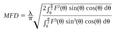
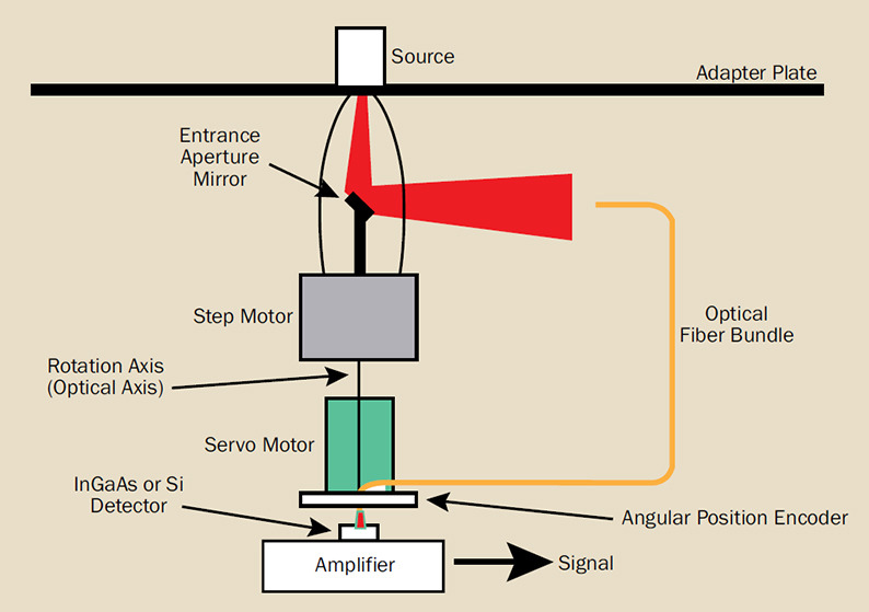
Instead, a scanning goniometric radiometer profiler is used to profile the angular intensity distribution of the beam. From the measured angular distribution, MFD is calculated using the Petermann II integral, derived by Klaus Petermann in 1983:

where F(θ) is the far-field intensity as a function of the scanning angle. A scanning goniometric radiometer system (Figure 4) traditionally involves moving a detector slowly through an arc with the sample fixed to determine the far-field profile. However, in a few cases, the test source was moved and the detector kept fixed (Figure 5). One of the strengths of this technique is that it does not require careful mechanical positioning of the test source; for many scanning geometries, the mechanical positioning needs only to be precise to a millimeter. Since far-field profiling requires far less precision in sample alignment and positioning, it tends to be more repeatable and less user-dependent than near-field profiling. With the right far-field scanner, it’s also much faster than near-field profiling.

Figure 4. A goniometric radiometer system; here, both the sensor and test source are fixed, allowing for real-time scanning.
Figure 5. With a standard goniometric radiometer set-up, either the source or the detector moves.

A fast scanning goniometric radiometer developed by Guttman1 and supplied by Ophir uses a fiber bundle rotating about a turning mirror, with both the test source and the detector kept fixed. The rotating fiber bundle is geometrically equivalent to a point sensor scanning through an arc about the test source. To generate high-resolution far-field profile hemispheres, the folding mirror is rotated at increments to acquire profiles at different azimuthal angles, equivalent to rotating the test source. This process takes under a minute. This technique has been shown to be accurate in characterizing the MFD of H-66 Photonics Handbook 2016 Test & Measurement PS Nov. 2015 Measurement Feature Figure 4 Lisa Step Motor Rotation Axis (Optical Axis) Servo Motor InGaAs or Si Detector Amplifier Signal Source Adapter Plate Entrance Aperture Mirror Optical Fiber Bundle Angular Position Encoder Figure 4. A goniometric radiometer system; here, both the sensor and test source are fixed, allowing for real-time scanning. PS Nov. 2015 Measurement Feature Figure 5 Lisa r Source Detector Source Detector Stationary Source/Moving Detector Moving Source/Stationary Detector Figure 5. With a standard goniometric radiometer set-up, either the source or the detector moves.

Optical fibers and waveguides

Even for fibers with very small MFDs (<5 μm), non- Gaussian profiles and elliptical beam sizes were found to be reasonably characterized, transforming the far-field profile with the Petermann II integration, even though these attributes of the beams violated the assumptions of the Petermann II integral. Obtaining and understanding solid small beam profiling data can be challenging in work with optical systems. Such challenges can now be overcome, however, with these proven techniques.

Reference

1. J. Guttman, R. Chirita et al. (Sept. 26-28, 2000). A novel far-field scanning technique for rapid measurement of optical fiber parameters. Technical Digest: Symposium on Optical Fiber Measurements, ed. P.A. Williams and G.W. Day. As presented at the NIST Symposium on Optical Fiber Measurements (2000). Boulder, Colo. Open access: www.ophiropt.com/user_files/laser/beam_profilers/NIST2000_PAPER.pdf All images courtesy of Derrick Peterman/Ophir-Spiricon LLC

Contact Us illustration

Have questions? Require assistance?

Click below to to contact Ophir Photonics and we'll get back with you shortly.

Contact Ophir Photonics